Building a map from distances between cities
A nice student-size project for playing with non-linear optimization and the optimize module of scipy. This exercice may follow any introduction to gradient descent, line search, conjugate gradient etc. You will find one here (with nice Javascript animations!).
In order to be realistic, let’s use the googlemaps module to fetch the city coordinates and compute all the distances.
Note that the point here is to forget the coordinates as soon as we have the distances.
cities = """
Amsterdam Athens    Barcelona Berlin   Bucarest  Budapest Brussels Copenhagen
Dublin    Edinburgh Gibraltar Helsinki Istanbul  Kiev     Lisbon   London
Madrid    Milan     Moscow    Munich   Nantes    Oslo     Paris    Prague
Reykjavik Riga      Rome      Sofia    Stockholm Toulouse Vilnius  Warsaw
"""

cities = cities.split()
n = len(cities) # 32
Preparing the data
Below is a script to fetch the coordinates from Google Maps API.
You may need to get your own API key (exactly 40 characters long and starting with AIza) as explained on their Github page.
University campuses are often hidden behind proxies. You can set it up here with the snippet in comment.
import googlemaps

proxy_dict = {}  # from home

# if you need to set the proxy
# proxy_dict = { 'proxies': {"http": ">>>> fill here <<<<",
#                            "https": ">>>> fill here <<<<"} }

# Be careful, your API key is:
#   - is exactly 40 characters long
#   - starts with AIza
client = googlemaps.Client(key=">>>> fill in your API key <<<<",
                           requests_kwargs=proxy_dict)

coords = [client.geocode(c) for c in cities]
coords = [c[0]['geometry']['location'] for c in coords]

# Quick check...
coords[:3]
[{'lat': 52.3702157, 'lng': 4.895167900000001},
 {'lat': 37.9838096, 'lng': 23.7275388},
 {'lat': 41.3850639, 'lng': 2.1734035}]
By exploring the cities sorted by longitude, we can first notice that Copenhagen and Rome are almost aligned on the same meridian.
# Determine which cities are aligned on longitude
sort_lng = sorted(range(n), key = lambda i: coords[i]['lng'])
for i in sort_lng[14:20]:
    print ("{:>15} {:.4f}".format(cities[i], coords[i]['lng']))
           Oslo 10.7522
         Munich 11.5820
           Rome 12.4964
     Copenhagen 12.5683
         Berlin 13.4050
         Prague 14.4378
This fact will help us rotate the map in a familiar direction.
Now we can compute the distance matrix and forget about the coords.
import numpy as np
import numpy.linalg as la

# https://github.com/xoolive/geodesy/
import geodesy.wgs84 as geo

# compute the distance matrix
distances = np.array([[geo.distance(*x.values(), *y.values())
                       for x in coords] for y in coords])

# normalize the distance matrix
distances /= la.norm(distances)
np.save("cities_distances.npy", distances)
If you cannot find your way through the Google Maps API or with the geodesy package, you will find in distances.npy a binary representation of the normalized matrix to be loaded.
distances = np.load("cities_distances.npy")
The optimisation problem
We consider a matrix of distances separating cities in Europe. We want to find they (x,y)-positions on a map such that all distances are respected.
This corresponds to minimising the sum
\[f\left(x_0, y_0, \cdots, y_n\right) =\sum_i\sum_j \left(\left(x_i - x_j\right)^2 + \left(y_i - y_j\right)^2 - d_{i, j}^2\right)^2\]With 32 cities, that is a problem of 64 floating precision variables we can solve with many optimisation methods embedded in scipy.optimize.
We choose here fmin_bfgs (for Broyden-Fletcher-Goldfarb-Shanno), that takes the function to minimise and its derivate.
def func(*x):
    """ Compute the function to minimise.

    Vector reshaped for more readability.
    """
    res = 0
    x = np.array(x)
    x = x.reshape((n, 2))
    for i in range(n):
        for j in range(i+1, n):
            (x1, y1), (x2, y2) = x[i, :], x[j, :]
            delta = (x2 - x1)**2 + (y2 - y1)**2 - distances[i, j]**2
            res += delta**2
    return res

def func_der(*x):
    """ Derivative of the preceding function.

    Note: (f \circ g)' = g' \times f' \circ g
    Vector reshaped for more readability.
    """
    res = np.zeros((n, 2))
    x = np.array(x)
    x = x.reshape((n, 2))
    for i in range(n):
        for j in range(i+1, n):
            (x1, y1), (x2, y2) = x[i, :], x[j, :]
            delta = (x2 - x1)**2 + (y2 - y1)**2 - distances[i, j]**2
            res[i, 0] += 4 * (x1 - x2) * delta
            res[i, 1] += 4 * (y1 - y2) * delta
            res[j, 0] += 4 * (x2 - x1) * delta
            res[j, 1] += 4 * (y2 - y1) * delta
    return np.ravel(res)
Before we can call the BFGS algorithm, we need to compute an initial state. We use here a normal law but as we will want to plot the full convergence process later, we choose to scale the initial distribution of points with the norm of the distance matrix.
# initial random position
x0 = np.random.normal(size=(n, 2))

# normalize initial position so as to not look too stupid from start
l1, l2 = np.meshgrid(x0[:,0], x0[:,0])
r1, r2 = np.meshgrid(x0[:,1], x0[:,1])
x0 /= la.norm(np.sqrt((l1 - l2)**2 + (r1 - r2)**2))
So now we are ready!
import scipy.optimize as sopt
solution = sopt.fmin_bfgs(func, x0, fprime=func_der, retall=True)
Optimization terminated successfully.
         Current function value: 0.000000
         Iterations: 27
         Function evaluations: 28
         Gradient evaluations: 28
Post-processing the solution
Now we have a solution (which looks quite good!), and thanks to the retall parameter, we get the full convergence track in the second argument of the tuple.
Yet, since all rotations of maps and mirrors of solution maps are equivalent solutions to our problem (we call these symmetries), we need to do some post-processing to put the map in a familiar way:
- we can use the fact that Rome and Copenhagen are almost aligned to rotate the map;
- we take two cities that we know are east/west of each other, and decide whether a mirroring is necessary.
res = solution[0].reshape((n, 2))

# rotate it so that Copenhagen is above Rome
south, north = cities.index("Rome"), cities.index("Copenhagen")
d = res[north, :] - res[south, :]
rotate = np.arctan2(d[1], d[0]) - np.pi/2
mat_rotate = np.array([[np.cos(rotate), -np.sin(rotate)],
                       [np.sin(rotate), np.cos(rotate)]])
res = res @ mat_rotate  # matrix product, from Python 3.5

# mirror so that Reykjavik is west of Moscow
west, east = cities.index("Reykjavik"), cities.index("Moscow")
mirror = False
if res[west, 0] > res[east, 0]:
    mirror = True
    res[:, 0] *= -1

# apply the transformation to the full track
track = [p.reshape((n, 2)) @ mat_rotate for p in solution[1]]
if mirror == True:
    track = [p * np.array([-1, 1]) for p in track]
And now we can plot all cities coordinates with the track of convergence of their respective positions.
We manually set different parameters:
- we trim the image 10% outside the square hull of the cities’ positions;
- we use colormaps to put some sense in this spaghetti soup;
- we manually chose label placements so as to avoid overlaps and improve readability.
Note that this last item could be subject to automatic optimisation.
%matplotlib inline
import matplotlib.pyplot as plt
import matplotlib.cm as cm

fig = plt.figure()
fig.set_size_inches(7, 7)

ax = fig.gca()
ax.set_xticklabels([])
ax.set_yticklabels([])
ax.set_axis_off()

# Trimming the final image

bx = min(res[:, 0]), max(res[:, 0])
dx = bx[1] - bx[0]
ax.set_xlim(bx[0] - .1*dx, bx[1] + .1*dx)

by = min(res[:, 1]), max(res[:, 1])
dy = by[1] - by[0]
ax.set_ylim(by[0] - .1*dy, by[1] + .1*dy)

# label placement: subject to automatic optimization!
from collections import defaultdict
d = defaultdict(lambda: {'ha': "left", 'va': "bottom"})

for city in ["Barcelona", "Berlin", "Bucarest", "Budapest",
             "Istanbul", "Prague", "Reykjavik", "Sofia", ]:
    d[city] = {'ha': "left", 'va': "top"}
for city in ["Athens", "London", "Munich",  "Milan",
             "Stockholm", ]:
    d[city] = {'ha': "right", 'va': "top"}
for city in ["Copenhagen", "Dublin", "Edinburgh", "Gibraltar",
             "Helsinki", "Lisbon", "Madrid", "Nantes", "Oslo",
             "Paris", "Toulouse", ]:
    d[city] = {'ha': "right", 'va': "bottom"}

# automatic colouring
colors = cm.rainbow(np.linspace(0, 1, n))

for i, ((x, y), city, color) in enumerate(zip(res, cities, colors)):
    t = np.array([t[i, :] for t in track])
    ax.plot(t[:, 0], t[:, 1], color=color, alpha=.2)
    ax.scatter(x, y, color=color)
    ax.annotate("  " + city + "  ", (x, y), **d[city])
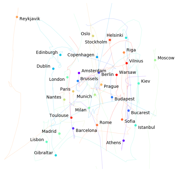
Now that we got it, we can work on our geography skills!


